Predicting Multiple Sclerosis with a Deep Learning Model

What is Multiple Sclerosis?

Multiple Sclerosis (MS) is a chronic condition where the body's immune system mistakenly attacks the protective covering of nerves in the brain and spinal cord. This damage interferes with how the nervous system communicates, leading to symptoms like muscle weakness, vision problems, numbness, and difficulty with coordination. MS can appear in different forms, sometimes as sudden episodes that come and go, and other times as a steady progression over time. While its exact cause remains uncertain, factors like genetics, environment, and immune-system dysfunction are all believed to play a role. There's currently no cure, but early detection and timely intervention can make a significant difference in managing the disease.

Clinically Isolated Syndrome & MS progression

For many patients, MS begins with a single neurological episode known as Clinically Isolated Syndrome (CIS). This initial attack, caused by inflammation or demyelination in the central nervous system, affects around 85% of those who eventually develop MS. However, not all CIS cases progress, and conversion rates vary widely. Identifying which early signs in CIS patients are likely to lead to MS is crucial for timely treatment decisions. This dataset explores those predictors to help anticipate and manage the risk of progression.

The data comes from a prospective study of Mexican mestizo patients recently diagnosed with CIS, collected at the National Institute of Neurology and Neurosurgery (NINN) in Mexico City between 2006 and 2010, and available on Kaggle.

Citation. Pineda, B., & Flores Rivera, J. D. J. (2023). Conversion predictors of Clinically Isolated Syndrome to Multiple Sclerosis in Mexican patients: a prospective study. Mendeley Data, V1. doi:10.17632/8wk5hjx7x2.1

What you'll learn in this walkthrough

Before we dive into the code, it helps to get a quick overview of the journey ahead. This walkthrough is divided into four key stages, each building toward the final goal of predicting MS using real patient data.

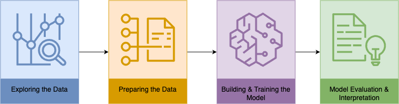
Stage 1 · Exploring the data

Before jumping into any modeling, it's important to spend time with the data and really understand what each feature represents and how it behaves. Visualising the inputs helps spot patterns, strange outliers, or missing values that could throw off the results later. In medical datasets especially, every column could reflect something meaningful, like a symptom or a diagnostic clue, so it's not just about cleaning the data, it's about respecting it. Exploring the data up front gives your model a better shot at learning something real and reliable.

1.1 Explaining the dataset features

1. Age. Patient age in years. MS typically begins between 20 and 50. Age helps identify early onset, predict progression, and tailor treatment strategies.
2. Schooling. Years the patient spent in school. Often used as a proxy for socioeconomic status, which can influence access to healthcare, nutrition, and environmental exposure. The evidence is inconclusive, but we include it in modeling.
3. Gender. MS affects women more often than men, especially in relapsing forms. Tracking gender helps understand risk patterns, disease behaviour, and treatment responses.
4. Breastfeeding. Some studies suggest being breastfed in infancy may offer slight protection against MS. The evidence is not conclusive, so it's an exploratory variable.
5. Varicella (chickenpox). Prior Varicella-zoster infection has been investigated as an environmental factor. Evidence is not conclusive; included to explore correlations.
6. Initial symptoms. Type of symptoms at the first neurological episode, categorised as Visual, Sensory, Motor and their combinations. The dataset records 15 distinct symptom combinations.
7. Mono- or poly-symptomatic. Whether the patient experienced a single symptom or multiple symptoms at the first episode, reflecting the severity and complexity of onset.
8. Oligoclonal bands (OCBs). Proteins in cerebrospinal fluid and a key marker of CNS inflammation. Their presence is strongly associated with MS.
9. LLSSEP / ULSSEP. Lower- and upper-limb somatosensory evoked potentials. Abnormal results indicate disruption in nerve pathways.
10. VEP. Visual evoked potentials; measures the brain's response to visual stimuli and flags demyelination along the visual pathway.
11. BAEP. Brainstem auditory evoked potentials; detects abnormalities in the auditory pathways.
12. Periventricular, Cortical, Infratentorial & Spinal-cord MRI. Lesion markers across brain regions; several are strongly associated with MS.
13. Initial & Final EDSS. Expanded Disability Status Scale (0 to 10) at diagnosis and at end of follow-up; used to assess severity and progression.
14. Group (target). Whether a CIS patient converted to Clinically Definite MS (CDMS). Group 1 = CDMS, Group 2 = non-CDMS. This is what the models predict.

We'll now visualise the impact of the important features on the final outcome, the Group classification as CDMS or non-CDMS.

1.2 Understanding gender trends

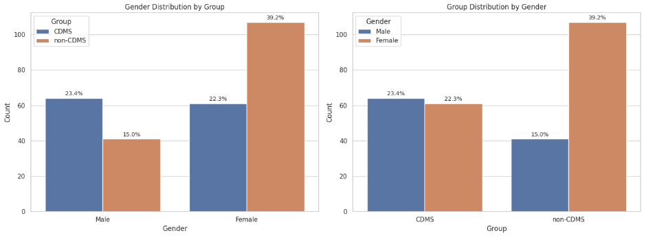
Males appear slightly more likely to progress from CIS to CDMS in this dataset, while females (more prevalent overall) show a higher presence in the non-CDMS category. This seems to contradict the well-established finding that MS is more common in females, but a few factors matter: this specific Mexican mestizo cohort may not reflect global trends; not all females who present with CIS convert within the study period, while males (though fewer) may progress faster; and progression timelines vary widely between 2006 and 2010. It's a reminder to weigh context and local population dynamics when interpreting medical data.

1.3 Exploring age trends

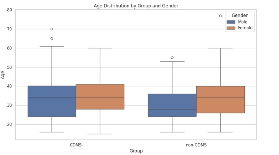
CDMS tends to occur at slightly higher ages, though the difference is not dramatic. Age is not a sharp separator on its own, but it may still hold predictive signal, especially in combination with other features.

1.4 Understanding breastfeeding trends

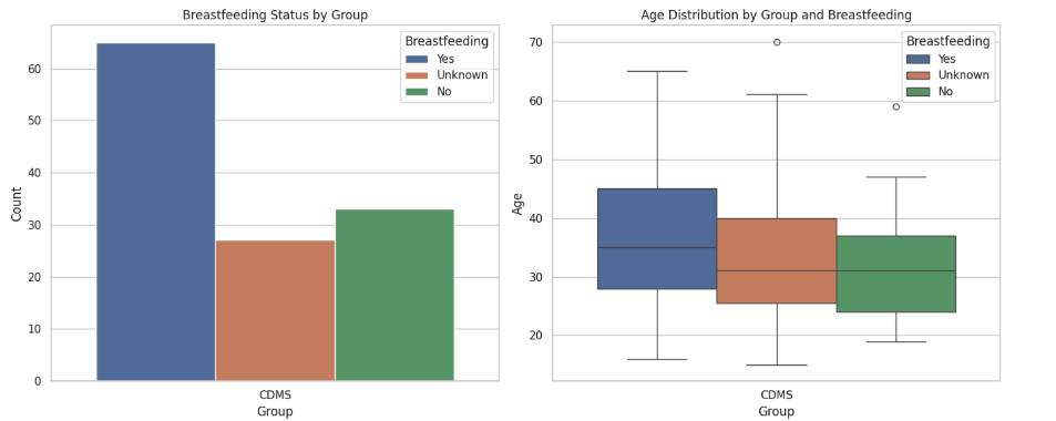
A majority of CDMS patients were breastfed, followed by smaller "unknown" and "non-breastfed" groups. This might seem counterintuitive given the assumption that breastfeeding could be protective, but it doesn't imply causation, it simply reflects that most patients in this dataset were breastfed. The age distribution across breastfeeding status shows no stark difference, though the breastfed group has a slightly wider spread with some older outliers.

1.5 Exploring varicella (chickenpox) trends

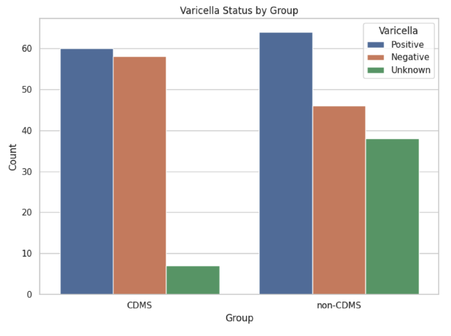
While Varicella has been hypothesised to influence immune response and possibly MS risk, this dataset doesn't show a strong or clear distinction between positive and negative cases across CDMS outcomes. It remains a relevant feature to include in predictive modeling, especially in combination with other clinical variables.

1.6 How initial symptoms shape MS progression

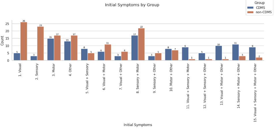
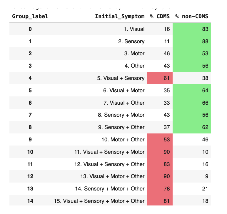
The bar chart and percentage table together offer a compelling view of how a patient's first neurological symptoms correlate with conversion to CDMS. Simple symptoms like visual or sensory alone are overwhelmingly seen in non-CDMS cases (83% of visual-only and 88% of sensory-only patients did not convert). In contrast, polysymptomatic onsets, especially those involving three or more symptom categories, are strongly associated with CDMS. This supports the clinical hypothesis that a more widespread or complex symptom presentation at onset may indicate a higher risk of progression.

1.7 Oligoclonal band presence across groups

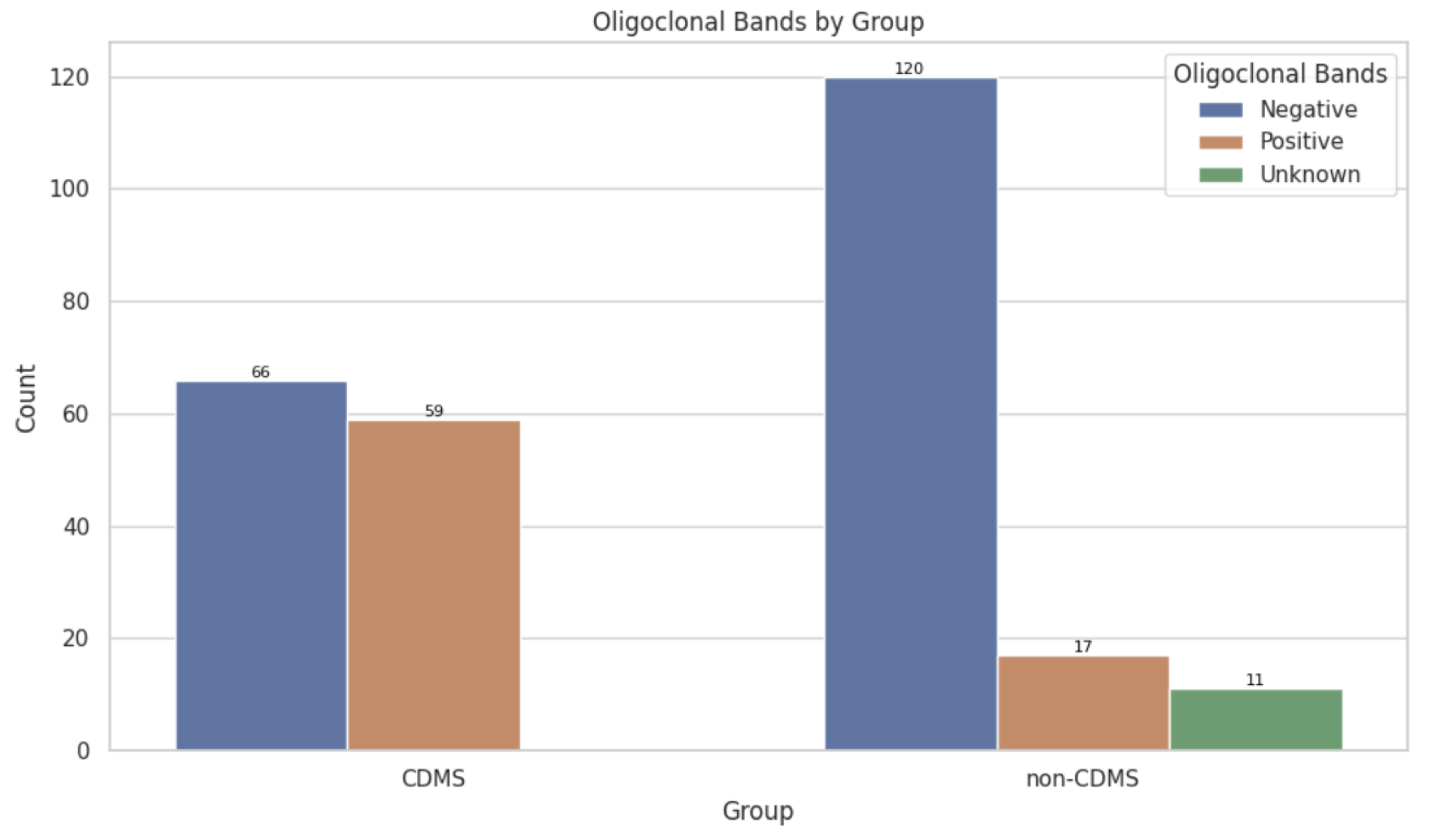
While OCB positivity is relatively balanced in the CDMS group, the non-CDMS group is dominated by OCB-negative patients. This sharp contrast suggests a negative OCB status may be associated with a lower risk of MS progression, reinforcing the role of OCBs as a useful early predictor. We'll observe the feature importance of OCB during the neural-network predictions.

1.8 Diagnostic value of evoked-potential tests

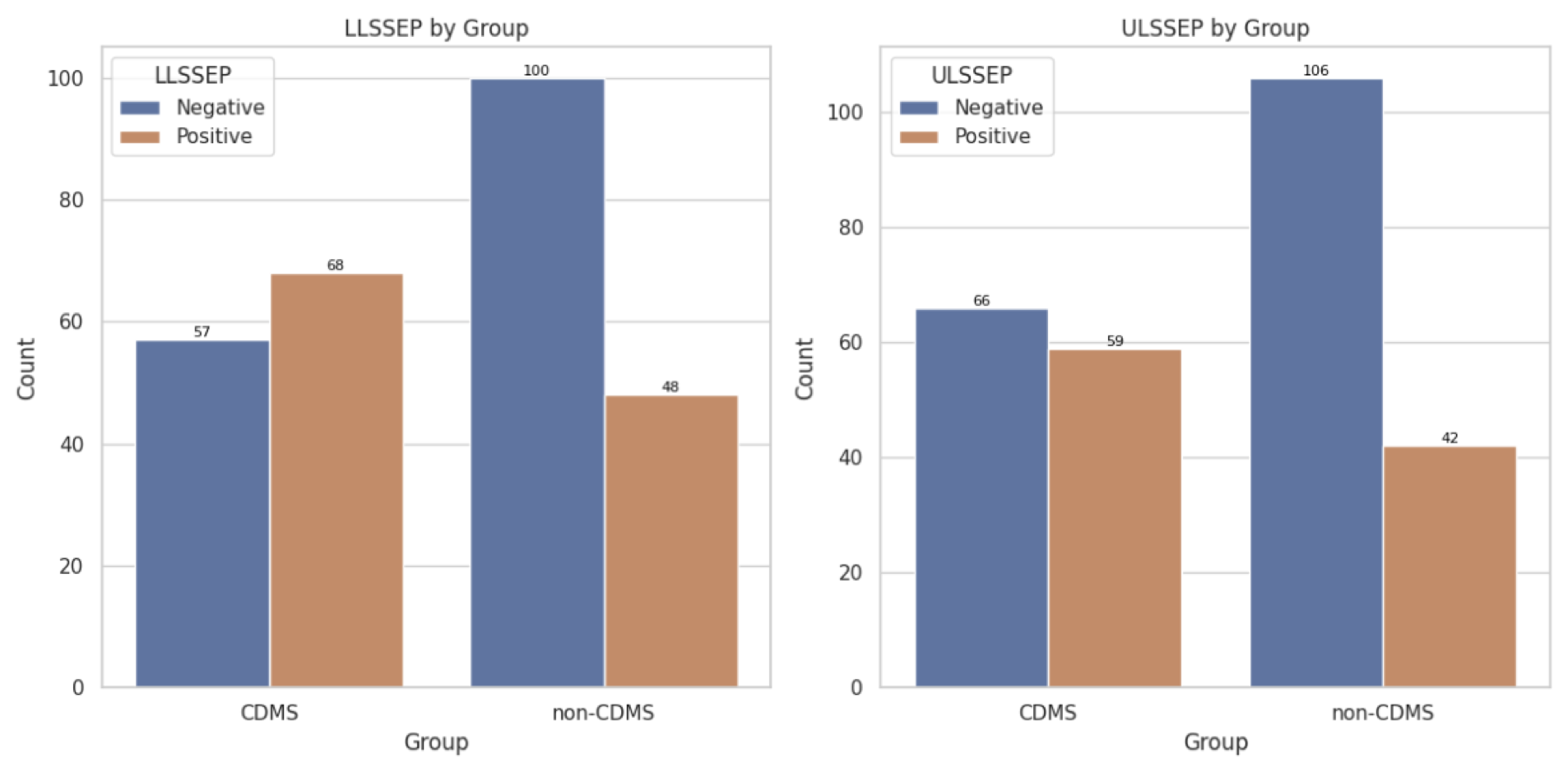
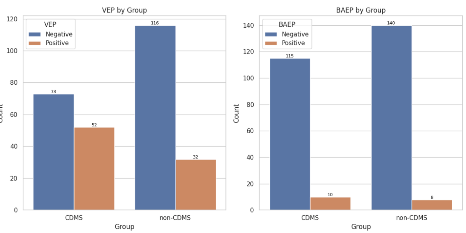
What is the Chi-Square test? A statistical method that checks whether two categorical variables are related (for example, "Positive" vs "Negative" test results across "CDMS" vs "non-CDMS"). A p-value below 0.05 means the difference is likely not due to chance.

Among the evoked-potential tests, LLSSEP, ULSSEP and VEP clearly differentiate CDMS from non-CDMS (p < 0.01), while BAEP lacks discriminatory power (p ≈ 0.54). These sensory pathways carry real predictive signal for progression.

1.9 MRI patterns as predictive indicators

We study all four MRI variables:

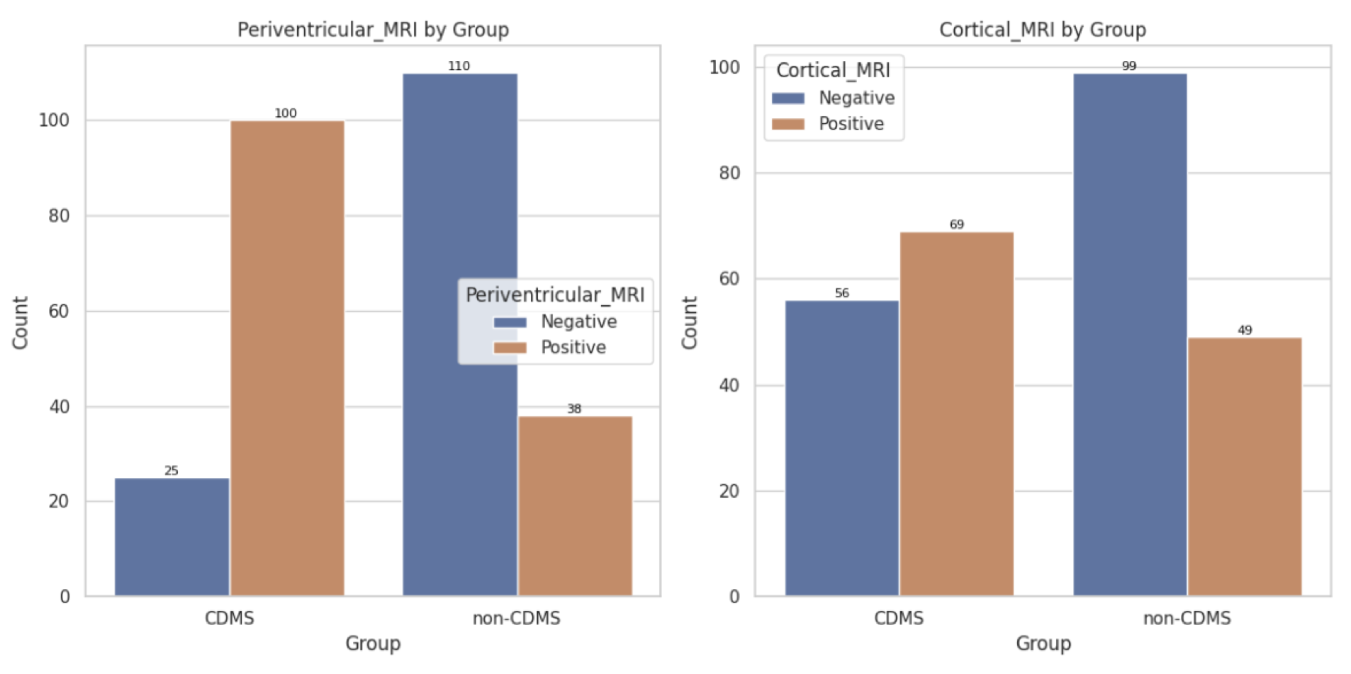
• Periventricular MRI: highly significant (Chi² = 77.85, p ≈ 0.0000).
• Cortical MRI: significant (Chi² = 12.59, p ≈ 0.0004).
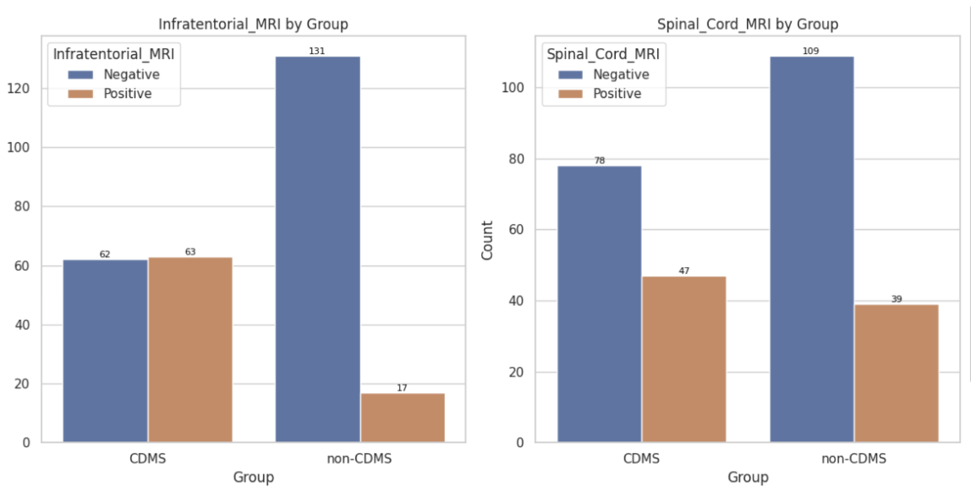
• Infratentorial MRI: highly significant (Chi² = 47.67, p ≈ 0.0000).
• Spinal-cord MRI: shows a trend but isn't conclusive (Chi² = 3.47, p ≈ 0.0625).

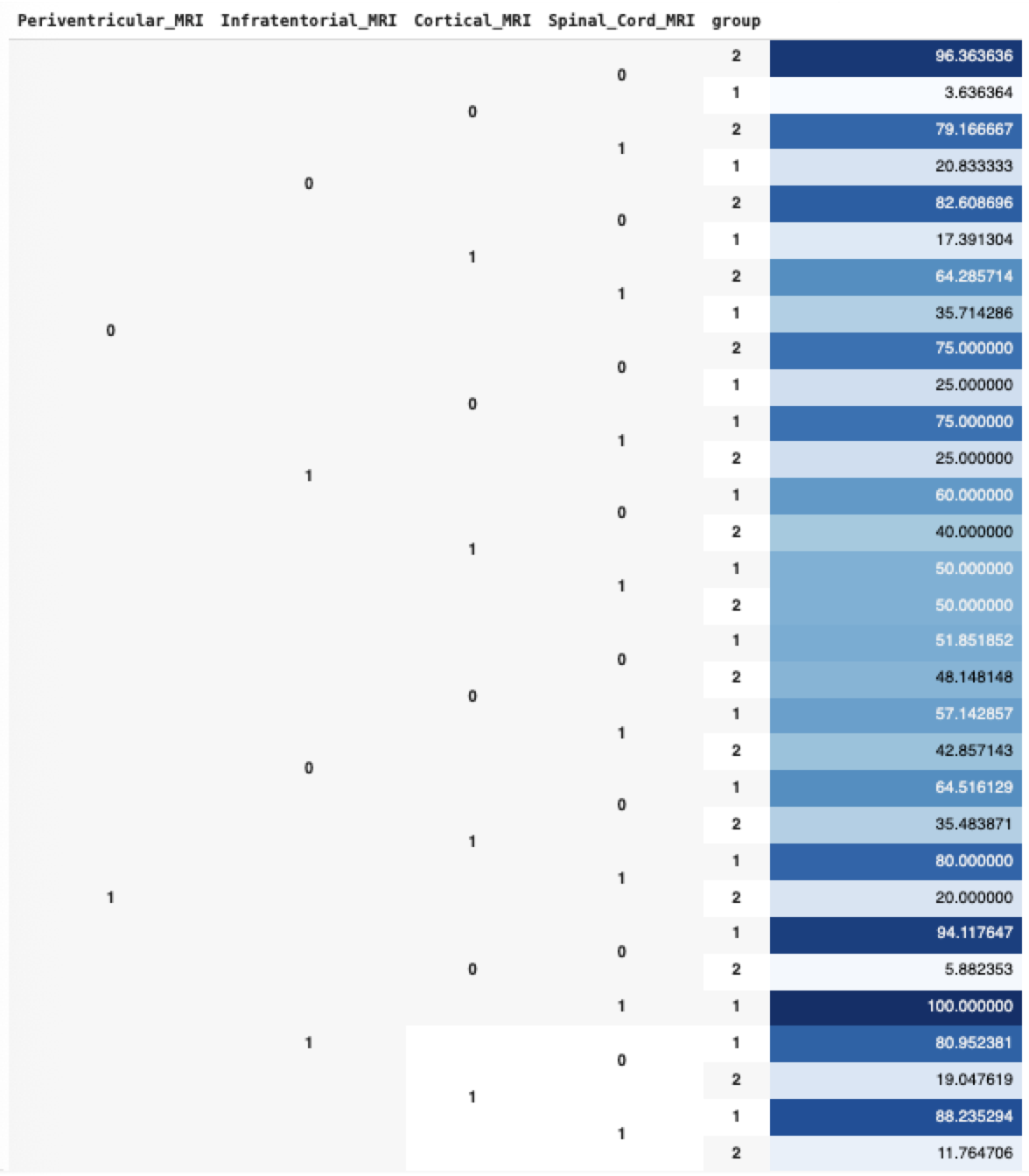
Testing positive on all MRI parameters is associated with an 88% likelihood of a CDMS diagnosis. Here is a combined view across all MRIs.

Stage 2 · Preparing the data

Now let's move on to the coding part and begin data preparation with Python. We load the CSV, drop rows missing the target, recode the group from 1/2 to 1/0, remove unused columns, split into features and target, impute missing values with column means, convert to tensors, and make an 80/20 train/validation split.

import torch
import torch.nn as nn
from torch.utils.data import DataLoader, TensorDataset
from sklearn.model_selection import train_test_split
from sklearn.metrics import accuracy_score, precision_score, recall_score, f1_score
import torch.optim as optim
import xgboost as xgb
import numpy as np
import pandas as pd
import seaborn as sns
import matplotlib.pyplot as plt

# Load dataset
df = pd.read_csv('sample_data/ms_data.csv')

# Drop rows with missing target, recode CDMS=1 / non-CDMS=0
df = df.dropna(subset=['group'])
df['group'] = df['group'].replace({2: 0})

# Remove unused columns (EDSS unavailable for CDMS cases)
df = df.loc[:, ~df.columns.str.contains('^Unnamed')]
df = df.drop(columns=['No', 'Initial_EDSS', 'Final_EDSS'], errors='ignore')

# Feature / target split, impute, tensors
X = df.drop(columns=['group']).fillna(df.mean())
y = df['group']
X_tensor = torch.tensor(X.values).float()
y_tensor = torch.tensor(y.values).long()

# 80 / 20 train-validation split
X_train, X_val, y_train, y_val = train_test_split(
    X_tensor, y_tensor, test_size=0.2, random_state=42)

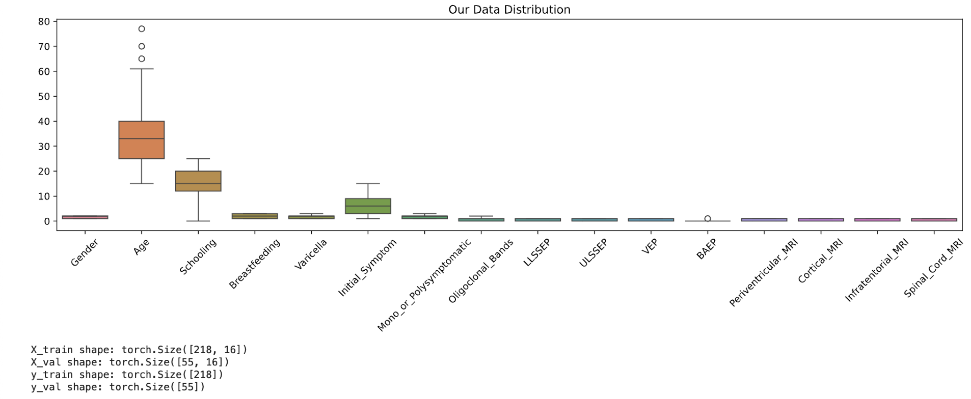
The plot below shows the feature distribution after preprocessing. We've skipped z-scoring since it's mainly relevant for continuous variables like Age and Schooling and has limited impact here. The number of features is reduced from 19 to 16, and a total of 218 rows are used for processing.

Stage 3 · Building & training the model

We build a Feed-Forward Neural Network (FFN) to classify our data into two categories (CDMS vs non-CDMS).

3.1 The model architecture

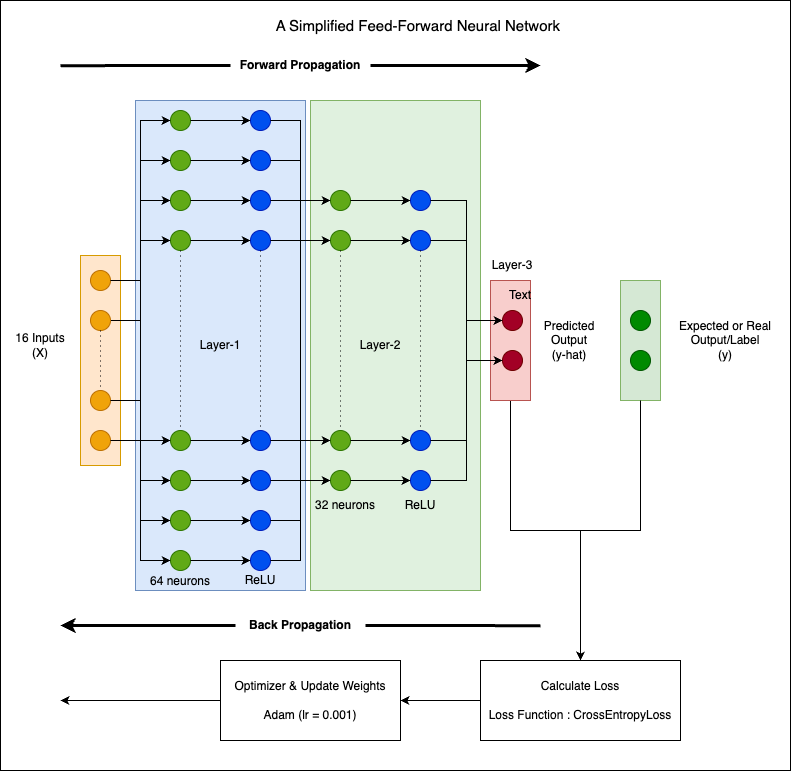
The model has three layers. The first takes all 16 input features through a dense (linear) layer with 64 neurons, followed by a ReLU activation. The second reduces this to 32 neurons, again with ReLU. The final layer maps those 32 values to 2 output logits, one per class.

What is ReLU? ReLU (Rectified Linear Unit) is an activation function that introduces non-linearity by keeping positive values and setting negatives to zero, letting the network learn complex patterns.

To train the model we use CrossEntropyLoss, a standard choice for classification that measures how far the predicted class probabilities are from the true labels.

What does the loss function do? A loss function like CrossEntropyLoss compares the predicted probabilities with the actual label and calculates how "wrong" the prediction is. The more incorrect the prediction, the higher the loss. Training aims to minimise it.

We use the Adam optimizer (learning rate 0.001), which adjusts learning dynamically and is well-suited to sparse or noisy gradients.

What is the role of an optimizer? The optimizer is the model's coach during training. When the network makes a prediction, the loss function says how wrong it was, and the optimizer tweaks the internal weights to reduce that error. Over many iterations, these small changes add up and the model becomes more accurate.

The training loop runs for 1,500 epochs. In each epoch we reset gradients, feed the data forward to get predictions, compute the loss, backpropagate, and update the weights. The loss is printed every 10 epochs to track progress.

3.2 Code for building & training the FFN

class FFN(nn.Module):
    def __init__(self, input_dim):
        super(FFN, self).__init__()
        self.network = nn.Sequential(
            nn.Linear(input_dim, 64),
            nn.ReLU(),
            nn.Linear(64, 32),
            nn.ReLU(),
            nn.Linear(32, 2)
        )
    def forward(self, x):
        return self.network(x)

model = FFN(X_train.shape[1])
lossfun = nn.CrossEntropyLoss()
optimizer = optim.Adam(model.parameters(), lr=0.001)

# Train for 1500 epochs
loss_history = []
for epoch in range(1500):
    model.train()
    optimizer.zero_grad()
    outputs = model(X_train)
    loss = lossfun(outputs, y_train)
    loss.backward()
    optimizer.step()
    loss_history.append(loss.item())
    if epoch % 10 == 0:
        print(f"Epoch {epoch}, Loss: {loss.item():.4f}")

3.3 Key observations

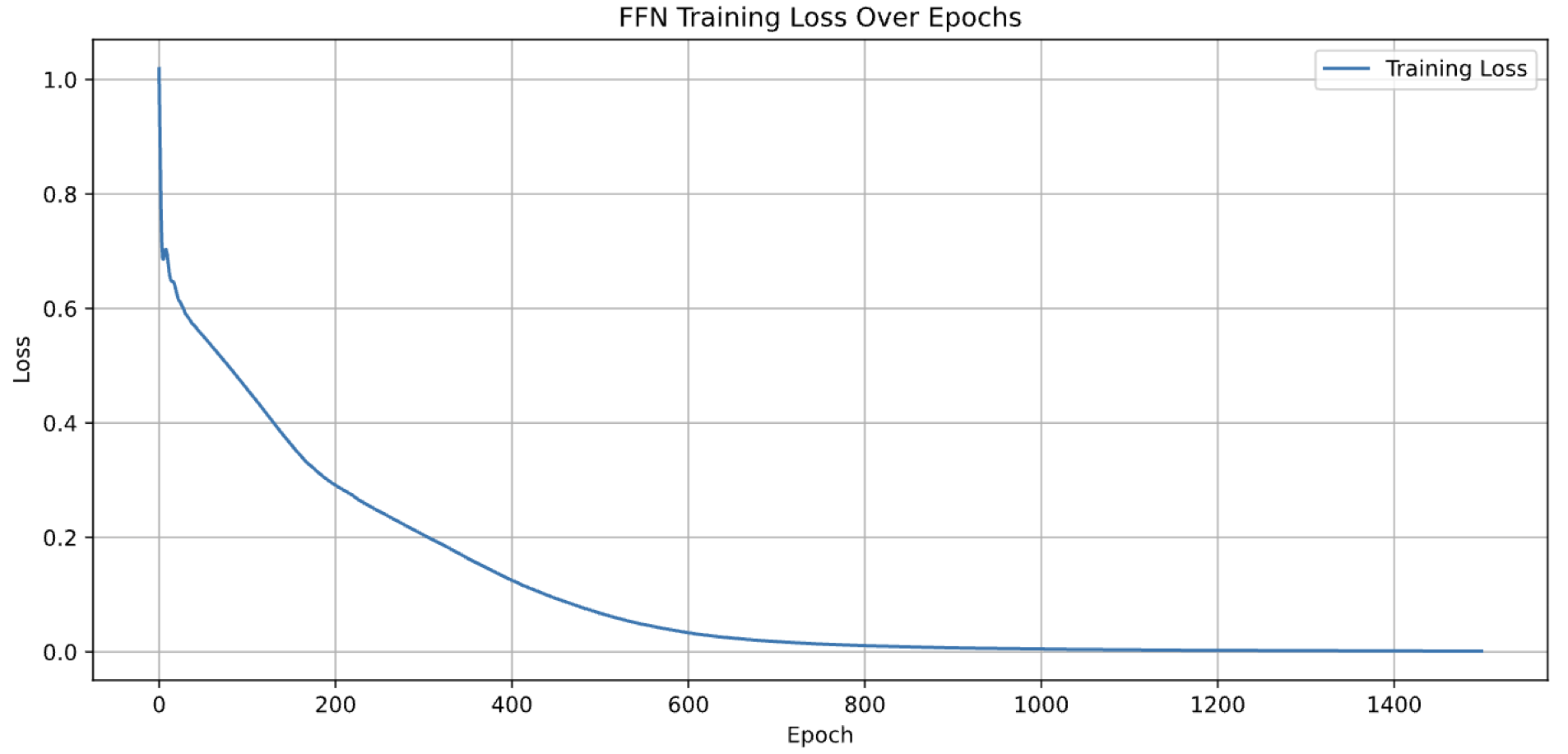
• Steady decrease in loss: training loss drops consistently from ~1.0 to near 0.0, indicating the model is learning and making fewer mistakes.
• Rapid early learning: most of the reduction happens in the first 300 to 500 epochs, as the model quickly adjusts its weights.
• Convergence: beyond ~700 epochs the loss plateaus, suggesting the model has reached an optimal state.

The curve is smooth and consistently declining, with no signs of overfitting or instability.

Stage 4 · Model evaluation & interpretation

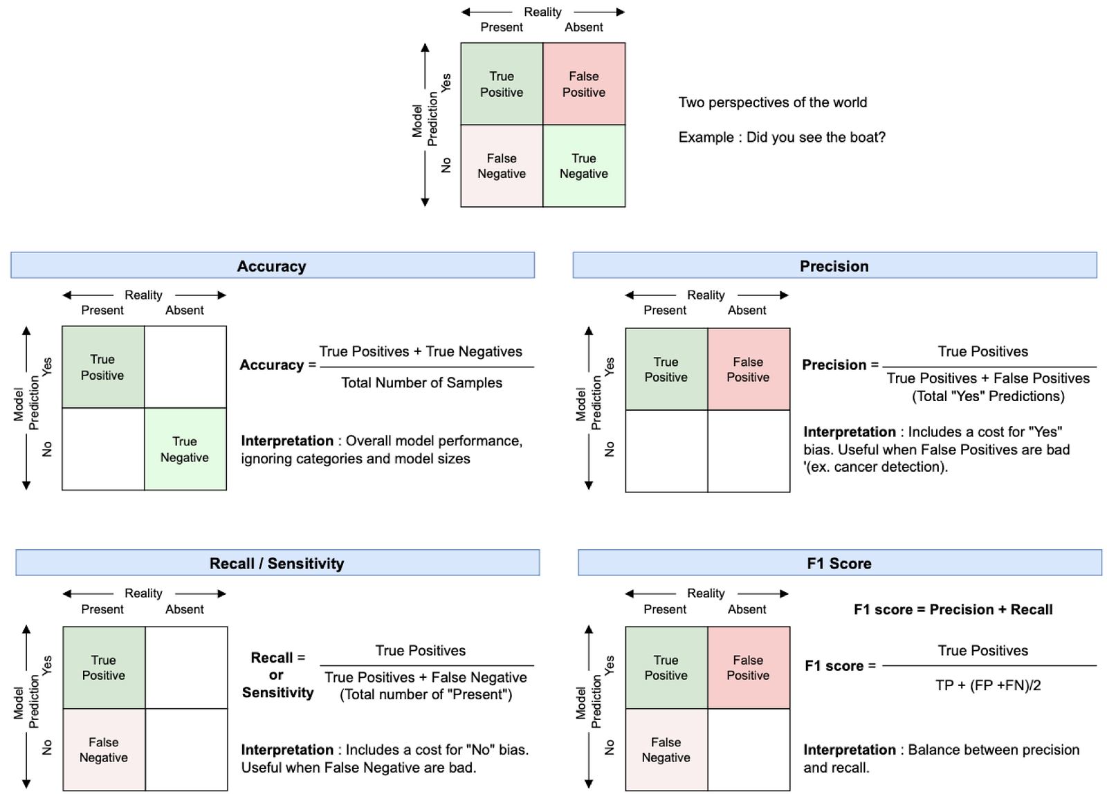
Model evaluation is usually based on four key metrics: Accuracy (the proportion of total predictions the model got right), Precision (of all predicted positives, how many were actually positive), Recall / Sensitivity (of all actual positives, how many were correctly predicted), and F1 Score (the harmonic mean of precision and recall).

4.1 Performance comparison: FFN vs XGBoost

Let's evaluate and compare these four metrics across two models: the Feed-Forward Neural Network (FFN) and XGBoost.

# Evaluate the FFN
model.eval()
with torch.no_grad():
    predictions = torch.argmax(model(X_val), axis=1)

print("FFN:", accuracy_score(y_val, predictions),
      precision_score(y_val, predictions),
      recall_score(y_val, predictions),
      f1_score(y_val, predictions))

# Train & evaluate XGBoost for comparison
X_tr, X_te, y_tr, y_te = train_test_split(X, y, test_size=0.2, random_state=42)
model_xgb = xgb.XGBClassifier(eval_metric='logloss')
model_xgb.fit(X_tr, y_tr)
preds_xgb = model_xgb.predict(X_te)

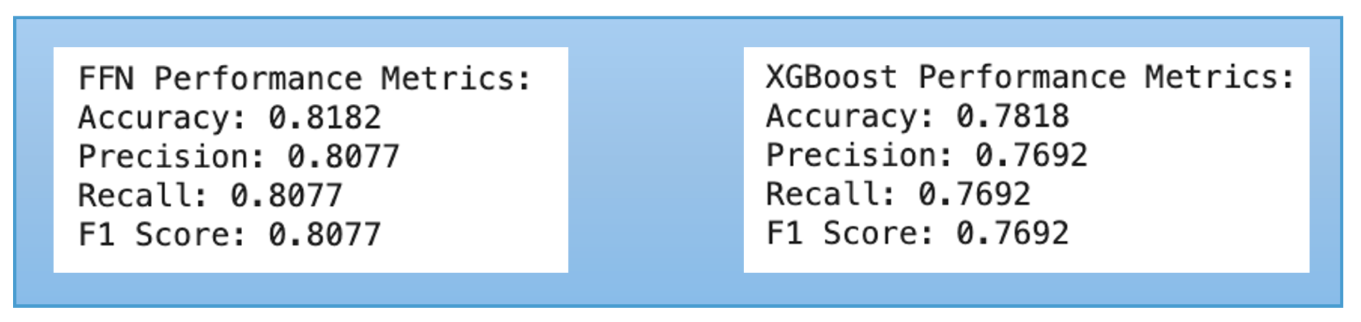
Result for FFN: Accuracy 80.82%, Precision 80.77%, Recall 80.77%, F1 80.77%. The FFN not only demonstrated higher accuracy but also struck an optimal balance between recall (correctly identifying true positives) and precision (minimising false positives), a crucial consideration in medical research where misclassification carries real consequences.

4.2 Feature importance (FFN model)

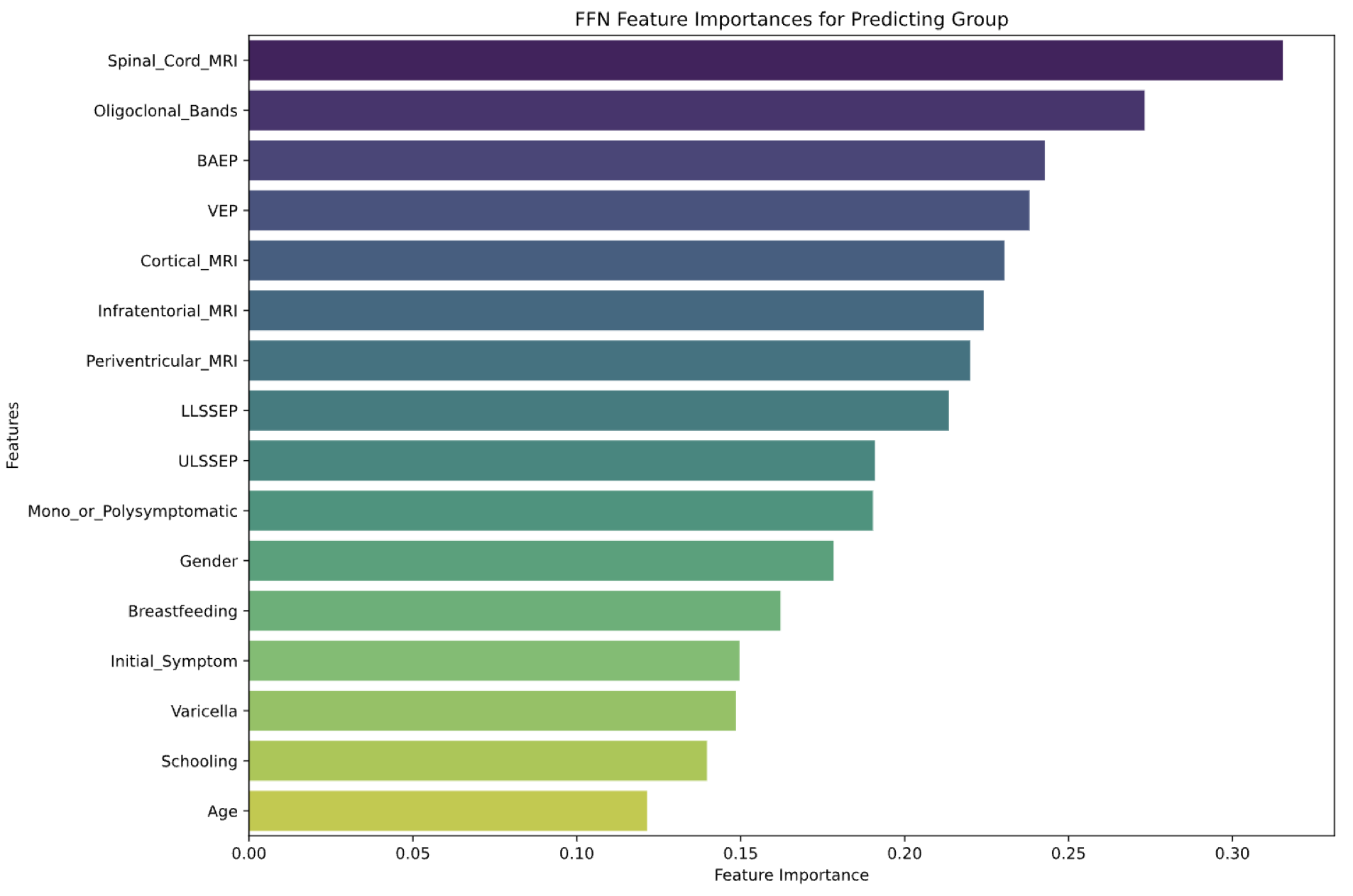
The learned feature importance validates the earlier statistical insights, the strong role of oligoclonal bands and specific MRI regions, reinforcing that neural networks can extract clinically meaningful patterns even from modestly sized datasets. Slight shifts (like Spinal-cord MRI ranking lower here) highlight the stochastic nature of neural-network training.

Wrapping it up

This study shows how deep learning can support complex medical predictions like MS diagnosis. By learning patterns across MRI findings, clinical features and test results, the model made classifications that align well with clinical expectations, a glimpse of AI's growing role in augmenting healthcare through decision-support, not replacement.

That said, performance is deeply tied to data quality and volume. This dataset was suitable for a proof of concept, but real-world deployment will require larger, diverse, clinically validated datasets. As we continue exploring AI in medicine, data integrity, ethics and clinical collaboration will be key to building solutions that are not only intelligent but reliable and responsible.